Composite Pulses
Composite pulses play a major role in NMR spectroscopy as they are the primary way in which experimental shortcomings resulting from RF and pulse length mis-calibration, field inhomogeniety and chemical shift offsets are compensated. I will some of the most basic aspects of these. This post is based on this classic review article by Malcolm Levitt from 1986.
import numpy as np
import matplotlib.pyplot as plt
from matplotlib import animation
from IPython.display import Image
from scipy.linalg import expm

from tins import spinsys
from bloch import Bloch
I = spinsys(0.5)
def ideal_pulse(start, phase, angle):

    phase = phase * np.pi / 180
    angle = angle * np.pi / 180
    axes = np.cos(phase) * I.x + np.sin(phase) * I.y
    Rot = expm(-1j * angle * axes)

    return Rot.conjugate().transpose() @ start @ Rot
Composite $\pi$ Pulse
The first composite pulse that we will explore is the first-ever composite pulse discovered. This is the classic $(\pi/2)_y (\pi)_x (\pi/2)y$ composite pulse to achieve inversion that is insensitive to both flip angle and RF power errors. First, I will make a function that will return the final state after executing this composite rotation for a given flip angle
def comp180_1(startop, flip):
    """ Composite π pulse: (π/2)y (π)x (π/2)y"""

    out = ideal_pulse(start=startop, phase=90, angle=flip)
    out = ideal_pulse(start=out, phase=0, angle=flip * 2)

    return ideal_pulse(start=out, phase=90, angle=flip)


def expect(detect, state):
    return np.trace(detect @ state)
Then, I collect the final state for series of pulses that are higher or lower that the ideal 90 pulse.
I do this for a single pulse as well
Then I collect the expectation values for the Ix Iy and Iz spin operators for the state at each point
pulses = [δ * 90 for δ in np.arange(0.5, 1.5, 0.01)]

comp = [comp180_1(I.z, τ) for τ in pulses]
onep = [ideal_pulse(I.z, 0, τ * 2) for τ in pulses]

comp_exp = np.array(
    [[expect(I.x, state), expect(I.y, state), expect(I.z, state)] for state in comp]
)

onep_exp = np.array(
    [[expect(I.x, state), expect(I.y, state), expect(I.z, state)] for state in onep]
)
fig, ax = plt.subplots(nrows=1, ncols=3, sharey=True, figsize=(8, 3), layout='constrained')

titles = [fr"$\langle \hat{{{i}}} \rangle$" for i in ["I_x", "I_y", "I_z"]]
for i in range(3):
    ax[i].plot(pulses, np.abs(comp_exp[..., i]), label="Composite", linewidth=2)
    ax[i].plot(pulses, np.abs(onep_exp[..., i]), label="Onepulse", linewidth=2)
    ax[i].set(ylabel=titles[i], ylim=(-0.1, 0.6))
    ax[i].yaxis.label.set_size(12)

ax[1].set_xlabel("Flip Angle (Ideal = $90^o$)", size=12)
ax[0].legend(frameon=False, fontsize=15)
ax[1].set_title("Composite π pulse: $(π/2)_y(π)_x(π/2)_y$", size=12)
plt.show()

def comp180_1_traj(start, flip):
    """
    trajectory for a particular flip angle
    """
    y901 = [ideal_pulse(start, 0, i) for i in np.linspace(0, flip, 10)]
    x180 = [ideal_pulse(y901[-1], 90, i) for i in np.linspace(0, flip*2, 20)]
    y902 = [ideal_pulse(x180[-1], 0, i) for i in np.linspace(0, flip, 10)]

    return y901 + x180 + y902
trajectories_composite = {}
for τ in np.linspace(75, 105, 10):
    trajectories_composite[τ] = comp180_1_traj(I.z, τ)

trajectories_single = {}
for τ in np.linspace(75, 105, 10):
    trajectories_single[τ] = [ideal_pulse(I.z, 0, pulse) for pulse in np.linspace(0, τ*2, 20)]

colors = [plt.cm.winter(i) for i in np.linspace(0, 1, len(trajectories_composite))]
%%capture
fig, (ax, ax1) = plt.subplots(ncols=2, figsize=(8, 4), subplot_kw={"projection": "3d"}, constrained_layout=True)
b = {}
b[0] = Bloch(axes=ax)
b[1] = Bloch(axes=ax1)
for k, i in b.items():
i.zlabel = "$I_z$", ""
i.xlabel = "$I_x$", ""
i.ylabel = "$I_y$", ""
i.frame_width = 2
i.sphere_alpha = 0.1
i.vector_width = 2
for axis in (ax, ax1):
axis.set_box_aspect([1, 1, 1])
def animate(i):
for k, v in b.items():
v.clear()
for c, (τ, traj) in enumerate(trajectories_composite.items()):
vector = [2 * expect(I.x, traj[i]), 2 * expect(I.y, traj[i]), 2 * expect(I.z, traj[i])]
b[0].add_vector(vector, color=colors[c])
for c, (τ, traj) in enumerate(trajectories_single.items()):
vector = [2 * expect(I.x, traj[i % 20]), 2 * expect(I.y, traj[i % 20]), 2 * expect(I.z, traj[i % 20])]
b[1].add_vector(vector, color=colors[c])
for k, v in b.items():
v.make_sphere()
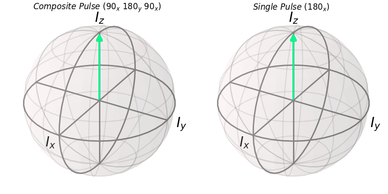
ax.set_title(r"$Composite\ Pulse\ (90_x\ 180_y\ 90_x)$")
ax1.set_title(r"$Single\ Pulse\ (180_x)$")
ax.set_facecolor = "white"
return [[ax, ax1]]
def init():
return [[ax, ax1]]
ani = animation.FuncAnimation(
fig, animate, range(40), init_func=init, blit=False, repeat=True,
)
ani.save("composite_1.gif", fps=15)
def comp90_1(startop, flip):
    ''' Composite π/2 pulse: (π/2)y (π/2)x '''

    out = ideal_pulse(startop, 90, flip)
    return ideal_pulse(out, 0, flip)
pulses = [δ * 90 for δ in np.arange(0.5, 1.5, 0.01)]

comp = [comp90_1(I.z, τ) for τ in pulses]
onep = [ideal_pulse(I.z, 0, τ) for τ in pulses]

comp_exp = np.array(
    [[expect(I.x, state), expect(I.y, state), expect(I.z, state)] for state in comp]
)

onep_exp = np.array(
    [[expect(I.x, state), expect(I.y, state), expect(I.z, state)] for state in onep]
)
fig, ax = plt.subplots(
    nrows=1, ncols=3, sharey=True, figsize=(6, 3), layout="constrained"
)

titles = ["Ix", "Iy", "Iz"]
for i in range(3):
    ax[i].plot(pulses, np.abs(comp_exp[..., i]), label="Composite", linewidth=2)
    ax[i].plot(pulses, np.abs(onep_exp[..., i]), label="Onepulse", linewidth=2)
    ax[i].set(ylabel=titles[i], ylim=(-0.1, 0.6))
    ax[i].yaxis.label.set_size(12)
    for border in ax[i].spines.values():
        border.set_linewidth(1)

ax[1].set_xlabel("Flip Angle (Ideal = $90^o$)")
ax[2].legend(frameon=False, fontsize=12)
fig.suptitle("Composite π/2 pulse: $(π/2)_y(π/2)_x$")
plt.show()

def comp90_1_traj(start, flip):
    y90 = [ideal_pulse(start, 0, i) for i in np.linspace(0, flip, 10)]
    x90 = [ideal_pulse(y90[-1], 90, i) for i in np.linspace(0, flip, 10)]

    return y90 + x90
trajectories_comp_90 = {}
for τ in np.linspace(75, 105, 10):
    trajectories_comp_90[τ] = comp90_1_traj(I.z, τ)

trajectories_single_90 = {}
for τ in np.linspace(75, 105, 10):
    trajectories_single_90[τ] = [
        ideal_pulse(I.z, 0, pulse) for pulse in np.linspace(0, τ, 10)
    ]

colors = [plt.cm.winter(i) for i in np.linspace(0, 1, len(trajectories_composite))]
%%capture
fig, (ax, ax1) = plt.subplots(
ncols=2, figsize=(8, 4), subplot_kw={"projection": "3d"}, constrained_layout=True
)
b = {}
b[0] = Bloch(axes=ax)
b[1] = Bloch(axes=ax1)
for k, i in b.items():
i.zlabel = "$I_z$", ""
i.xlabel = "$I_x$", ""
i.ylabel = "$I_y$", ""
i.frame_width = 2
i.sphere_alpha = 0.1
i.vector_width = 2
for axis in (ax, ax1):
axis.set_box_aspect([1, 1, 1])
def animate(i):
for k, v in b.items():
v.clear()
for c, (τ, traj) in enumerate(trajectories_comp_90.items()):
vec = [2 * expect(I.x, traj[i]), 2 * expect(I.y, traj[i]), 2 * expect(I.z, traj[i])]
b[0].add_vector(vec, color=colors[c])
for c, (τ, traj) in enumerate(trajectories_single_90.items()):
vec = [2 * expect(I.x, traj[i % 10]), 2 * expect(I.y, traj[i % 10]), 2 * expect(I.z, traj[i % 10])]
b[1].add_vector(vec, color=colors[c])
for k, v in b.items():
v.make_sphere()
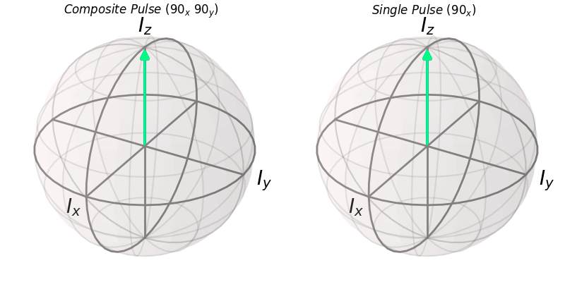
ax.set_title(r"$Composite\ Pulse\ (90_x\ 90_y)$")
ax1.set_title(r"$Single\ Pulse\ (90_x)$")
ax.set_facecolor = "white"
return [[ax, ax1]]
def init():
return [[ax, ax1]]
ani = animation.FuncAnimation(
fig,
animate,
np.arange(20),
init_func=init,
blit=False,
repeat=True,
)
ani.save("composite_90_1.gif", fps=15)
Q1
Make similar plots for the following composite pulses
- 90(180)-90(300) composite-90
- 90(0)-180(180)-270(0) composite-180
- 90(0)-200(90)-80(270)-200(90)-90(0) composite-180